Gradient Descent Traceback

Introduction

DEFINITION : In mathematics, gradient descent (also often called steepest descent) is a first-order iterative optimization algorithm for finding a local minimum of a differentiable function. The idea is to take repeated steps in the opposite direction of the gradient (or approximate gradient) of the function at the current point, because this is the direction of steepest descent. Conversely, stepping in the direction of the gradient will lead to a local maximum of that function; the procedure is then known as gradient ascent. (From wikipedia)_

Demonstrating gradient descent traceback in the simple case of polynomial functions with several examples:

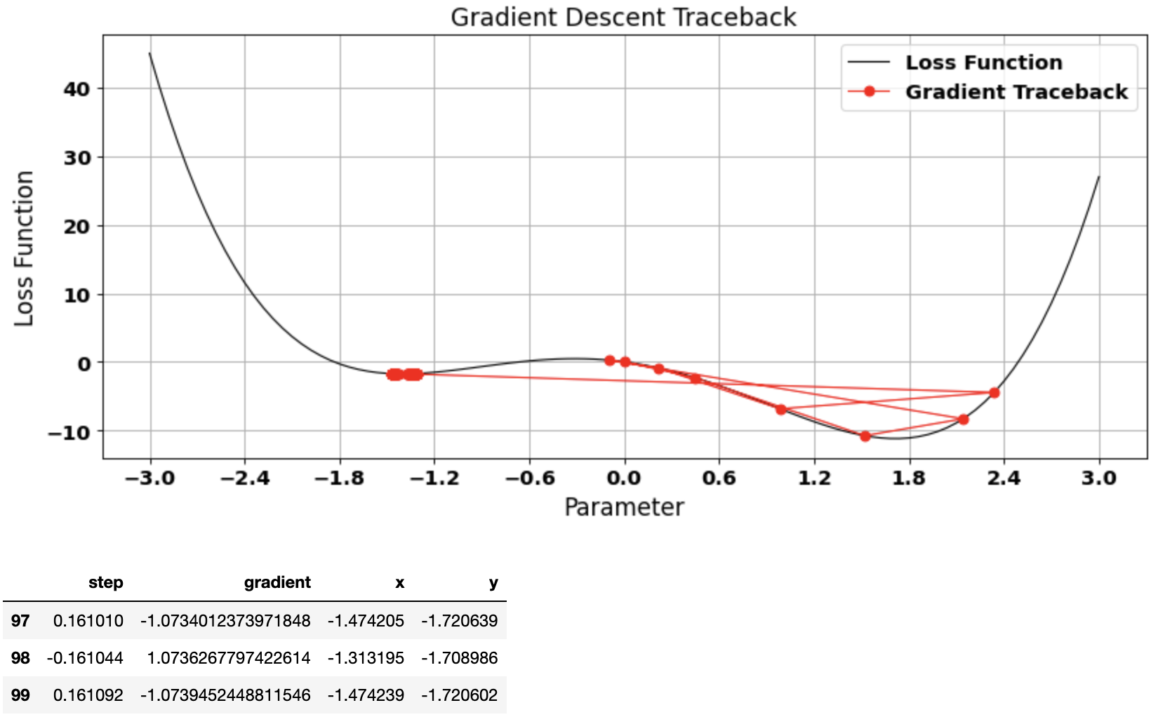
• Too large learning rate may cause the gradient descent algorithm to make huge jumps and miss the global minima
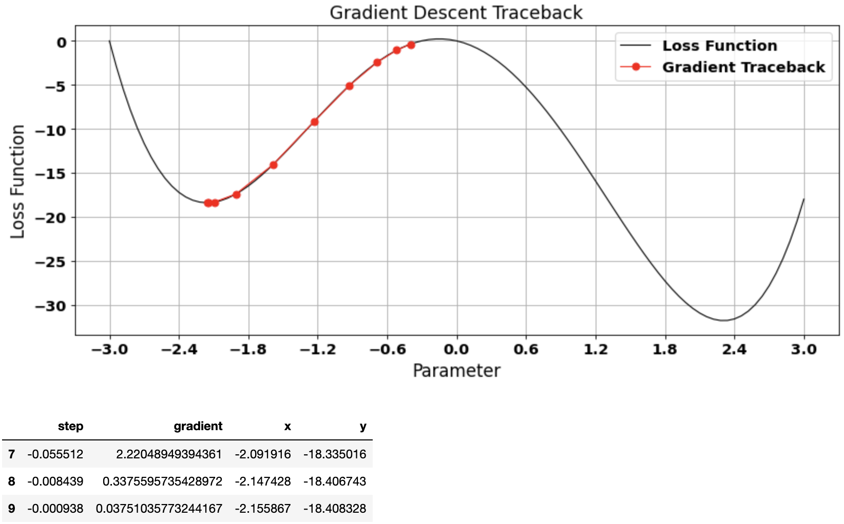
• Choice of starting point also influences whether gradient descent algorithm converges to local or global minima
• Too large or too small learning rate may cause the gradient descent algorithm to take drastically large number of epochs to converge

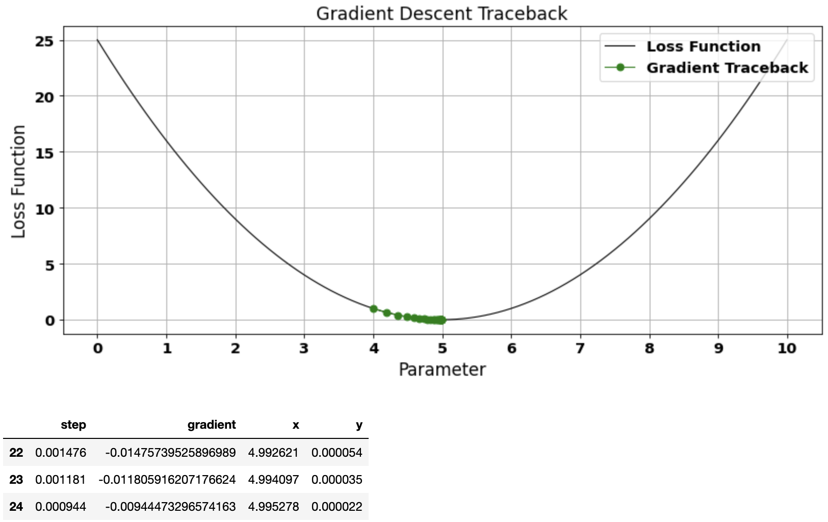
Example 1: Simple parabola

Simple parabola with just one minima

x = np.linspace(0, 10, num=101) #define the range of parameter values or x

def func(x): return (5 - x)**2 #define the loss function or y
y = func(x) #use the function to generate the loss for each choice of parameter 

function_df = pd.DataFrame({'x':x, 'y':y})

vector, gradient_df = gradient_descent(start=4.0, learn_rate=0.1)
plot_gradient_traceback(loss_function = function_df, gradient_path = gradient_df, location=1)
gradient_df.tail(3)

Example 2: Too large learning rate

Too large learning rate may cause the gradient descent algorithm to make huge jumps and miss the global minima

x = np.linspace(-3.0, 3.0, num=101) #define the range of parameter values or x

def func(x): return x**4 - 5*x**2 - 3*x #define the loss function or y
y = func(x) #use the function to generate the loss for each choice of parameter

function_df = pd.DataFrame({'x':x, 'y':y})

vector, gradient_df = gradient_descent(start=0.0, learn_rate=0.15)
plot_gradient_traceback(loss_function = function_df, gradient_path = gradient_df, location=1, color_traceback='red')
gradient_df.tail(3)

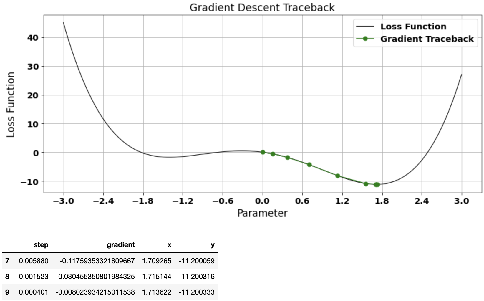
vector, gradient_df = gradient_descent(start=0.0, learn_rate=0.05)
plot_gradient_traceback(loss_function = function_df, gradient_path = gradient_df, location=1)
gradient_df.tail(3)

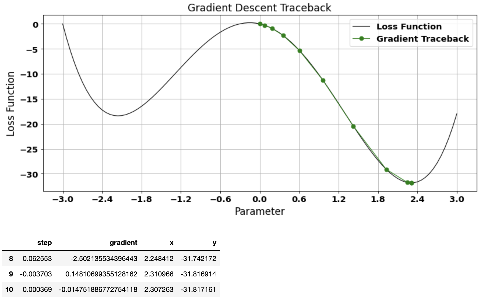
Example 3: Choice of starting point

Choice of starting point also influences whether gradient descent algorithm converges to local or global minima

x = np.linspace(-3.0, 3.0, num=101) #define the range of parameter values or x

def func(x): return x**4 - 10*x**2 - 3*x #define the loss function or y
y = func(x) #use the function to generate the loss for each choice of parameter

function_df = pd.DataFrame({'x':x, 'y':y})

vector, gradient_df = gradient_descent(start=-0.4, learn_rate=0.025)
plot_gradient_traceback(loss_function = function_df, gradient_path = gradient_df, location=1, color_traceback='red')
gradient_df.tail(3)

vector, gradient_df = gradient_descent(start=0.0, learn_rate=0.025)
plot_gradient_traceback(loss_function = function_df, gradient_path = gradient_df, location=1)
gradient_df.tail(3)

Example 4: Too many epochs

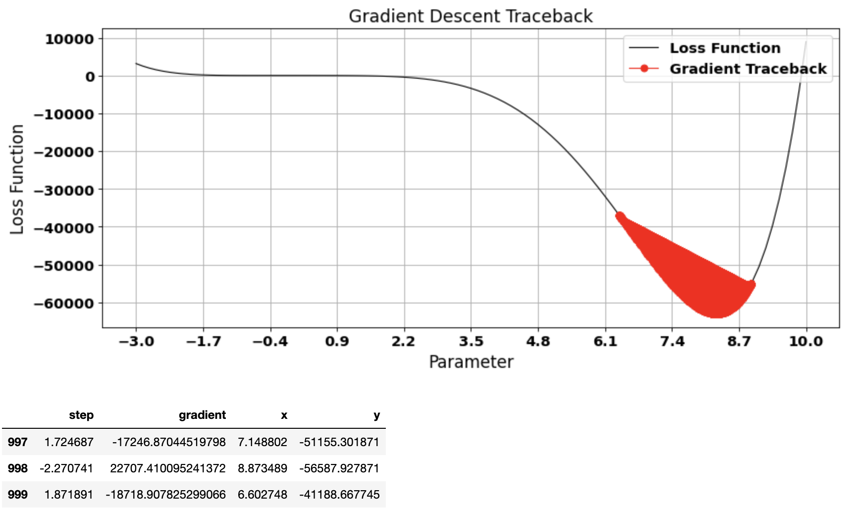
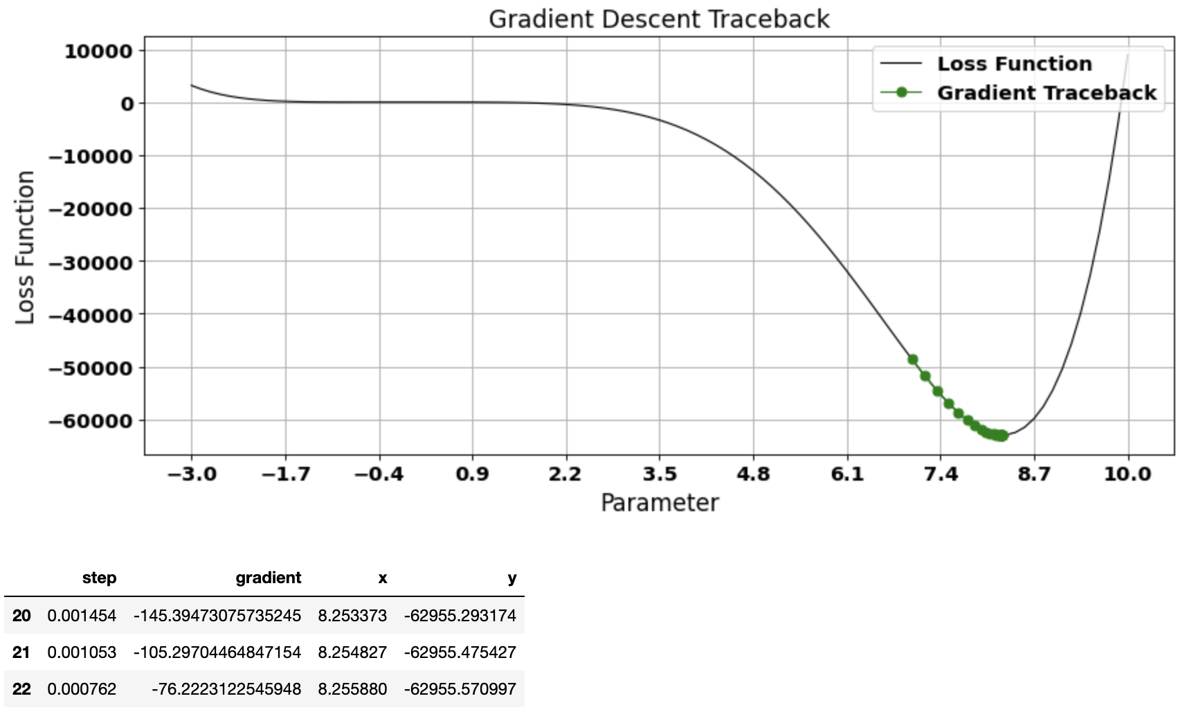
Too large or small learning rate may cause the gradient descent algorithm to take drastically large number of epochs to converge

x = np.linspace(-3.0, 10.0, num=101) #define the range of parameter values or x

def func(x): return x**6 -10*x**5 + x**4 - 10*x**2 - 3*x #define the loss function or y
y = func(x) #use the function to generate the loss for each choice of parameter

function_df = pd.DataFrame({'x':x, 'y':y})

Couldn’t converge in even 1000 epochs with a large learn_rate of 0.0001

vector, gradient_df = gradient_descent(start=7.0, learn_rate=0.0001, n_iter=1000)
plot_gradient_traceback(loss_function = function_df, gradient_path = gradient_df, location=1, color_traceback='red')
gradient_df.tail(3)

Could converge in just 23 epochs with a smaller learn_rate of 0.00001

vector, gradient_df = gradient_descent(start=7.0, learn_rate=0.00001)
plot_gradient_traceback(loss_function = function_df, gradient_path = gradient_df, location=1)
gradient_df.tail(3)

Appendix

Required Libraries

import pandas as pd
import numpy as np
import numdifftools as nd
import matplotlib as mpl
import matplotlib.pyplot as plt
from matplotlib.pyplot import figure

Define a function to calculate gradients, steps, update parameter, corresponding loss and record it in a dataframe for every iteration / epoch:

def gradient_descent(start, learn_rate, n_iter=100, tolerance=0.001, gradient = lambda x: nd.Gradient(func)([x]) ):
    gradient_df = pd.DataFrame(columns = ['step', 'gradient', 'x', 'y'])
    vector = start
    for _ in range(n_iter):
        step = -learn_rate * gradient(vector)
        #gradient = Delta(y) for a small change in x / Delta(x)
        #then take the absolute
        gradient_df = gradient_df.append({'step' : step, 'gradient' : gradient(vector), 'x' : vector, 'y' : func(vector)}, ignore_index=True)
        if np.all(np.abs(step) <= tolerance):
            break
        vector += step
    return vector, gradient_df

Define a function to plot the gradient descent traceback:

def plot_gradient_traceback(loss_function, gradient_path, location = 4, color_traceback = 'green'):
    font = {'weight' : 'bold',
            'size'   : 13}
    
    mpl.rc('font', **font)
    
    figure(figsize=(12, 5), dpi=80)
    
    plt.plot(loss_function.x, loss_function.y, color = 'black', label = "Loss Function", linewidth = 1)
    plt.plot(gradient_path.x, gradient_path.y, color = color_traceback, label = "Gradient Traceback", marker='o', linewidth = 1)
    plt.legend(loc=location)
    
    plt.ylabel('Loss Function', fontsize=15)
    plt.xlabel('Parameter', fontsize=15)
    
    plt.xticks(function_df.x[0::10])
    plt.title('Gradient Descent Traceback')
    plt.grid(True)
    plt.show()