Anti Money Laundering (AML) / Fraud Detection

Introduction

1. What is Money Laundering? (wiki)

Money laundering is the process of concealing the origin of money, obtained from illicit activities such as drug trafficking, corruption, embezzlement or gambling, by converting it into a legitimate source.

(1.1) Money Laundering Steps (wiki)

• the first involves introducing cash into the financial system by some means (“placement”);
• the second involves carrying out complex financial transactions to camouflage the illegal source of the cash (“layering”);
• and finally, acquiring wealth generated from the transactions of the illicit funds (“integration”).

(1.2) Domain Knowledge (read)

Indicators of suspicious activity:

• Substantial increases in cash deposits of any individual or business without apparent cause
• Deposits subsequently transferred within a short period out of the account and to a destination not normally associated with the customer
• Deposit and withdrawal transactions conducted in cash rather than through forms of debits and credits
• Large cash withdrawals from a previously dormant/inactive account, or from an account which has just received an unexpected large credit from abroad
• Large number of individuals making payments into the same account without an adequate explanation

2. Dataset Overview (kaggle)

Paysim synthetic dataset of mobile money transactions. Each step represents an hour of simulation. This dataset has over 6M transactions and for purposes of illustration we will sample a subset of 100K transactions for model building. (use this smaller sample to work through our problem before fitting a final model on all of data)

aml_data = pd.read_csv('PS_20174392719_1491204439457_log.csv', sep=',')
aml_data = aml_data.sort_values(by = ['nameDest','step']).reset_index(drop=True)
aml_data = aml_data.head(100000)
aml_data.head()

(2.1) Dataset Exhibit

step	type	amount	nameOrig	oldbalanceOrg	newbalanceOrig	nameDest	oldbalanceDest	newbalanceDest	isFraud	isFlaggedFraud
352	CASH_IN	156985.310	C1180747031	36186.000	193171.310	C1000004082	0.000	0.000	0	0
354	CASH_OUT	228252.330	C1978911345	953.000	0.000	C1000004082	0.000	228252.330	0	0
370	TRANSFER	1331742.990	C1539355936	11088.000	0.000	C1000004082	228252.330	1559995.310	0	0
374	CASH_OUT	363030.740	C1680720313	19486.000	0.000	C1000004082	1559995.310	1923026.060	0	0
379	CASH_IN	156015.830	C1185840905	55451.000	211466.830	C1000004082	1923026.060	1767010.230	0	0

3. Exploratory Data Analysis

(3.1) Describe

aml_data.describe().T.style.format("{:,.0f}")

column	count	mean	std	min	25%	50%	75%	max
step	100,000	241	142	1	154	236	333	738
amount	100,000	261,876	675,325	4	76,767	159,810	279,180	51,990,861
oldbalanceOrg	100,000	1,226,464	3,493,829	0	0	17,310	190,918	49,585,040
newbalanceOrig	100,000	1,261,481	3,531,372	0	0	0	283,927	39,585,040
oldbalanceDest	100,000	1,620,428	3,599,760	0	146,642	564,907	1,700,329	152,338,227
newbalanceDest	100,000	1,803,755	3,889,847	0	228,118	703,375	1,898,856	152,338,227
isFraud	100,000	0	0	0	0	0	0	1
isFlaggedFraud	100,000	0	0	0	0	0	0	0

(3.2) Class Imbalance

isFraud : Only 0.2% of transactions are fraudulent

print("Value Count : isFraud\n\n")

c = aml_data[['isFraud']].value_counts(dropna=False)
p = aml_data[['isFraud']].value_counts(dropna=False, normalize=True)*100
print(pd.concat([c,p], axis=1, keys=['Count', 'Percentage']).reset_index())

isFraud	Count	Percentage
0	99,804	99.8
1	196	0.2

(3.3) Value Counts

(3.3.1) Transaction-type

type	Count	Percentage
CASH_OUT	53,245	53.2
CASH_IN	33,235	33.2
TRANSFER	12,560	12.6
DEBIT	960	1.0

(3.3.2) Transaction-type X isFraud

type	isFraud	Count	Percentage
CASH_OUT	0	53,151	53.2
CASH_IN	0	33,235	33.2
TRANSFER	0	12,458	12.5
DEBIT	0	960	1.0
TRANSFER	1	102	0.1
CASH_OUT	1	94	0.1

4. Feature Engineering

(Building Candidate Variables)

Creating the right expert / candidate variables is a critical step before we proceed to training our model. Encapsulating the problem dynamics as best as possible into these expert variables, prepares the data for the model in an as optimal way as possible. Refer

(4.1) Concat two or more identifiers for grouping (see code)

These features can help our model identify suspicious patterns like:

• frequent or large cash (or other) txns between an origin and dest account
• frequent or large cash (or other) txns from an origin account
• frequent or large cash (or other) txns to a dest account
• txns of amount just under the $10k reporting limit by federal law

nameOrig_nameDest	nameOrig_type	nameDest_type	nameOrig_nameDest_type
C1180747031_C1000004082	C1180747031_CASH_IN	C1000004082_CASH_IN	C1180747031_C1000004082_CASH_IN
C1978911345_C1000004082	C1978911345_CASH_OUT	C1000004082_CASH_OUT	C1978911345_C1000004082_CASH_OUT
C1539355936_C1000004082	C1539355936_TRANSFER	C1000004082_TRANSFER	C1539355936_C1000004082_TRANSFER

(4.2) Rolling frequency & amount (see code)

Can help track large or frequent txns to or from an account, account pair or identifier group.

(4.3) Time since last txn (see code)

Fast successive txns from the same account or identifier group can help track the 2nd stage of money laundering i.e. Layering.

(4.4) Velocity change (see code)

Can help track unusual behavior for an account, account pair or identifier group.

(4.5) Had previous fraud (see code)

Should ideally be blocked but just in case such account is still active.

(4.6) % Change in balance (see code)

Can help track sudden large deposits or withdrawal from an account.

5. Train Test Split

# drop identifiers
model_data = aml_data.drop(columns = ['nameOrig','nameDest','nameOrig_nameDest','nameOrig_type','nameDest_type','nameOrig_nameDest_type','isFlaggedFraud'])
model_data.head()

• We have lag based features so we can’t randomly sample train set.
• Instead should first sort by days.
• Here training on first 25 days.

train = model_data[model_data.day < 26].drop(['day'], axis=1)
train.head()

• Testing on remainder 5 days.

test = model_data[model_data.day >= 26].drop(['day'], axis=1)
test.head()

6. Model Pipeline

(6.1) Numerical Featurees

Tree based models don’t need normalization

numeric_pipeline = Pipeline(steps=[
    ('impute', SimpleImputer(strategy='mean')) #,('scale', MinMaxScaler())
])

(6.2) Categorical Features

categorical_pipeline = Pipeline(steps=[
    ('impute', SimpleImputer(strategy='most_frequent')),
    ('one-hot', OneHotEncoder(handle_unknown='ignore', sparse=False))
])

(6.3) Full Feature Processor

full_processor = ColumnTransformer(transformers=[
    ('number', numeric_pipeline, numerical_features),
    ('category', categorical_pipeline, categorical_features)
])

(6.4) Complete Model Pipeline

6.4.1 SelectFromModel for Feature Selection

For tabular large size data, tree boosting models generally work better than other models and require less data pre-processing. And CatBoost is the only model which can give XGBoost a run for its money but there aren’t many categorical features. So, we have narrowed our attempts for accuracy improvements to tuning XGBoost hyper-parameters while using different downsampling ratios.

xgb_model = xgboost.XGBClassifier(subsample=0.85, max_depth=15, learning_rate=0.3, objective= 'binary:logistic',n_jobs=-1,verbosity = 0)
xgb_pipeline = Pipeline(steps=[('preprocess', full_processor), ('feature_selection', SelectFromModel(xgboost.XGBClassifier())), ('model', xgb_model)])

7. Model Selection

(7.1) Rolling-window Cross-validation on Original Train Set

Try different XGBoost Hyper-parameters

Total instances 98625
Total positive instances 162
TimeSeriesSplit(gap=0, max_train_size=None, n_splits=5, test_size=None)
TRAIN: [    0     1     2 ... 16437 16438 16439] TEST: [16440 16441 16442 ... 32874 32875 32876]
TRAIN: [    0     1     2 ... 32874 32875 32876] TEST: [32877 32878 32879 ... 49311 49312 49313]
TRAIN: [    0     1     2 ... 49311 49312 49313] TEST: [49314 49315 49316 ... 65748 65749 65750]
TRAIN: [    0     1     2 ... 65748 65749 65750] TEST: [65751 65752 65753 ... 82185 82186 82187]
TRAIN: [    0     1     2 ... 82185 82186 82187] TEST: [82188 82189 82190 ... 98622 98623 98624]

Model	Iteration_count	Recall_mean	Recall_std	Fscore_mean	Fscore_std
xgb_V1	5	0.637	0.082	0.767	0.058
xgb_V2	5	0.660	0.073	0.785	0.050
xgb_V3	5	0.629	0.088	0.761	0.059
xgb_V4	5	0.660	0.073	0.782	0.050

(7.2) Rolling-window Cross-validation on Downsampled Train Set

Try different XGBoost Hyper-parameters & Downsampling-ratio for selected models

The xgb_v3 model with a downsampling ratio of 50:1 (original ratio is 500:1) gives best Recall & a good Fscore

print(xgb_model_V3.get_xgb_params())

subsample=0.9, max_depth=15, learning_rate=0.3, objective= 'binary:logistic',n_jobs=-1,verbosity = 0

Model	Downsample_Ratio	Iteration_count	Recall_mean	Recall_std	Fscore_mean	Fscore_std
xgb_V3	50	5	0.766	0.109	0.724	0.167
xgb_V2	50	5	0.754	0.120	0.722	0.174
xgb_V4	50	5	0.752	0.098	0.695	0.203
xgb_V1	50	5	0.750	0.132	0.709	0.208
xgb_V1	100	5	0.741	0.135	0.705	0.239
xgb_V3	150	5	0.739	0.169	0.674	0.280
xgb_V2	150	5	0.738	0.148	0.667	0.291
xgb_V4	150	5	0.738	0.148	0.692	0.279
xgb_V1	150	5	0.735	0.152	0.684	0.288
xgb_V4	100	5	0.731	0.143	0.731	0.196
xgb_V3	100	5	0.728	0.115	0.708	0.209
xgb_V2	100	5	0.722	0.101	0.717	0.233
xgb_V1	200	5	0.676	0.167	0.790	0.129
xgb_V4	200	5	0.672	0.174	0.767	0.110
xgb_V2	200	5	0.668	0.165	0.784	0.126
xgb_V3	200	5	0.660	0.173	0.774	0.138

(7.3) Train the selected model on full Train Set

# separate minority and majority classes
negative = train[train.isFraud==0]
positive = train[train.isFraud==1]

# downsample majority
neg_downsampled = resample(negative,
 replace=False, # sample without replacement to avoid overfittting                    
 n_samples=len(positive)*50, # match number in minority class
 random_state=27) # reproducible results

# combine majority and upsampled minority
downsampled = pd.concat([positive, neg_downsampled]).sort_values(by='step').reset_index(drop=True)

# check new class counts
downsampled.isFraud.value_counts()

xgb_model = xgboost.XGBClassifier(subsample=0.85, max_depth=15, learning_rate=0.3, objective= 'binary:logistic',n_jobs=-1,verbosity = 0)
xgb_pipeline = Pipeline(steps=[('preprocess', full_processor), ('feature_selection', SelectFromModel(xgboost.XGBClassifier())), ('model', xgb_model)])

x_train = downsampled.drop(['step','isFraud'], axis=1).fillna(0)
y_train = downsampled[['isFraud']]

x_test = test.drop(['step','isFraud'], axis=1).fillna(0)
y_test = test[['isFraud']]

8. Generalization Performance

Our choice of model evaluation metrics is Recall & Fscore because:

• Class Imbalance
• Cost of FN > Cost of FP

print('XGBoost Test Recall', round(recall_score(y_test, xgb_pipeline.predict(x_test)),3))
print('XGBoost Test F-Score', round(f1_score(y_test, xgb_pipeline.predict(x_test)),3))

XGBoost Test Recall 0.882
XGBoost Test F-Score 0.909

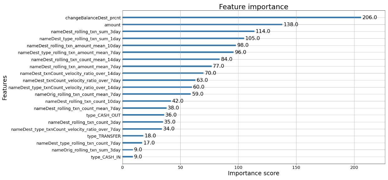
9. XGB feature importance

plot_importance(xgb_model)

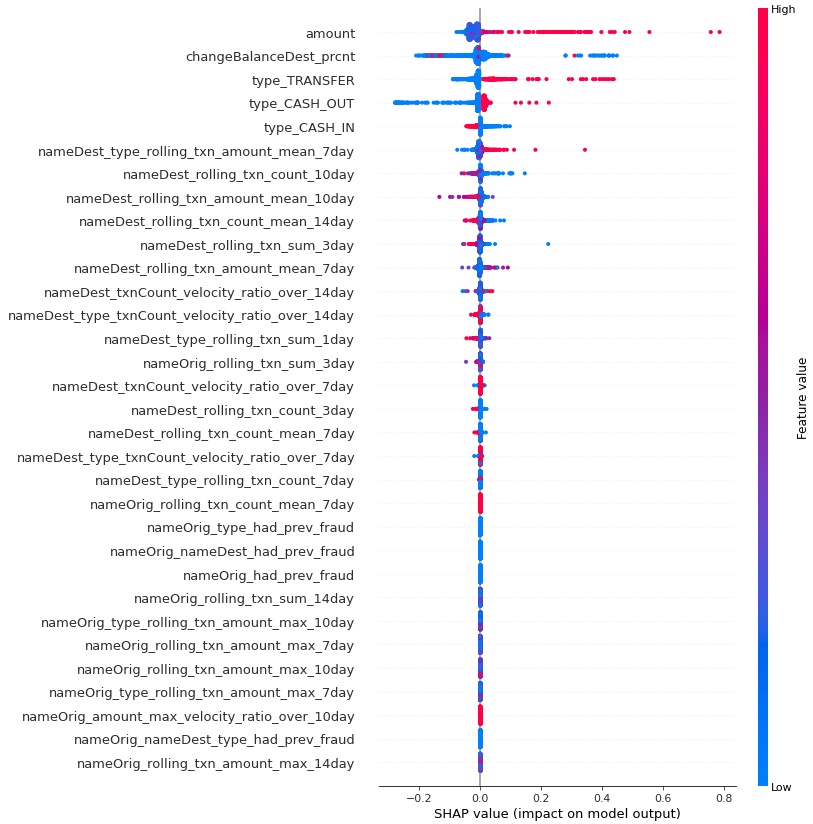
10. Model explainability

Shapley values for model explainability

(10.1) Overall shapley feature importance

shap.plots.beeswarm(shap_values_ebm)

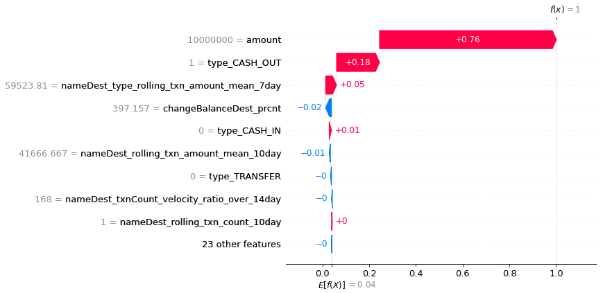
(10.2) Explaining a particular prediction

shap.plots.waterfall(shap_values_ebm[34]) #sample index

Appendix

(A.1) Dataset Dictionary

1. step - maps a unit of time in the real world. In this case 1 step is 1 hour of time. Total steps 744 (30 days simulation).
2. type - CASH-IN, CASH-OUT, DEBIT, PAYMENT and TRANSFER.
3. amount - amount of the transaction in local currency.
4. nameOrig - customer who started the transaction.
5. oldbalanceOrg - initial balance before the transaction.
6. newbalanceOrig - new balance after the transaction.
7. nameDest - customer who is the recipient of the transaction.
8. oldbalanceDest - initial balance recipient before the transaction. Note that there is not information for customers that start with M (Merchants).
9. newbalanceDest - new balance recipient after the transaction. Note that there is not information for customers that start with M (Merchants).
10. isFraud - This is the transactions made by the fraudulent agents inside the simulation. In this specific dataset the fraudulent behavior of the agents aims to profit by taking control or customers accounts and try to empty the funds by transferring to another account and then cashing out of the system.
11. isFlaggedFraud - The business model aims to control massive transfers from one account to another and flags illegal attempts. An illegal attempt in this dataset is an attempt to transfer more than 200.000 in a single transaction.

(A.2) Code

see code

(A.3) References

wiki

domain knowledge